Transportation Logistics

Resources

• Slides
• Exercise Questions 1 (Solution), Exercise Questions 2 (Solution)

Logistics is: The right product, at the right place, at the right time. Transportation problems solve the place.

Transportation Problems

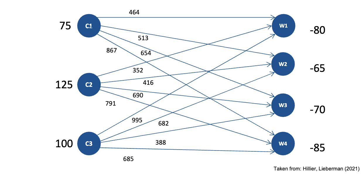
To facilitate supply network planning (decentralized global production planning), cross-docking, or the redistribution of empty containers or shared mobility systems, transportation problems can be solved using an optimization model:

• $n$ sources with capacity $a_i$
• $m$ sinks with demand $b_j$
• Transportation costs $c_{i,j}$ per unit from source $i$ to sink $j$
• Decision variable $x_{i,j}$: number of units transported from source $i$ to sink $j$
• Constraints on capacity and demand, and non-negativity of decision variables.
• The objective is to minimize total transportation costs:
  $\min {\sum }_{i=1}^n{\sum }_{j=1}^m{c}_{i,j}{x}_{i,j}$

This can generally be solved using Simplex or heuristic methods (north-west corner, matrix minimum).

Single-Route Optimization

Traveling Salesman (TSP)

The simplest transportation optimization problem. It doesn’t consider source/sink or capacity constraints, but rather the shortest route to visit all nodes (cities) and return to the starting point. Easy for small instances, but NP-hard for larger ones.

It minimizes the cost of trips $x_{i,j}$ from $i$ to $j$ with distances $c_{i,j}$:

$$\min C=\sum _{i=1}^n\sum _{j=1}^n{c}_{i,j}{x}_{i,j}$$

• where every location is reached and left: ${\sum }_{i=1}^n{x}_{i,j}=1\forall i$ and ${\sum }_{j=1}^n{x}_{i,j}=1\forall j$
• where subtours are eliminated (no smaller loops around position $z$): $z_i-z_j+n\cdot x_{i,j}\le n-1\forall i,j\in 2,...,n;i\ne j$
• where variables are binary: $x_{i,j}\in 0,1\forall i,j$

On paper, the traveling salesman can be solved using heuristics like nearest neighbor (start anywhere, then go to closest unvisited) or successive insertion (insert any unvisited node into the existing tour at the cheapest position). This solution can then be improved using 2-Opt.

Königsberg Bridge Problem

The problem of finding a walk through the city of Königsberg that would cross each of its seven bridges once and only once. It was solved by Euler in 1736, laying the foundation for graph theory.

Successive Insertion

A heuristic for constructing a tour by starting with a small subset of nodes and iteratively inserting the remaining nodes into the tour at the position that minimizes the increase in total distance.

Doing the process by hand is simple:

1. Start with a small tour (e.g., two nodes).
2. For each remaining node, calculate the cost of inserting it between every pair of consecutive nodes in the current tour.
3. Insert the node at the position that results in the smallest increase in total distance.
4. Repeat until all nodes are included in the tour.

2-Opt

An algorithm to iteratively improve a given route by removing two edges and reconnecting the two paths in a different way to reduce the total distance. The iteration stops when no further improvements can be made.

Two variants of 2-Opt exist:

• Steepest Descent: Optimize for the largest improvement in each iteration. First, all possible edge pairs are evaluated, and the best swap is performed.
• Decent Procedure: Optimize for the first improvement found. The algorithm stops as soon as a better solution is found, which is then used as the new starting point for the next iteration.

To perform 2-Opt by hand:

1. Start with an initial tour (e.g., from the nearest neighbor heuristic).
2. Identify all pairs of edges in the tour.
3. For each pair of edges, calculate the total distance if the edges are swapped (i.e., the two edges are removed and the two paths are reconnected in the opposite way).
4. If any swap results in a shorter total distance, perform the swap and update the tour.
5. Repeat steps 2-4 until no further improvements can be made.

Multi-Route Logistics

Vehicle Routing (VRP)

A generalization of the TSP where multiple vehicles are used to service a set of customers. Each vehicle has a capacity limit, and the goal is to minimize the total distance traveled while ensuring that all customer demands are met.
Each tour is performed by one vehicle and must start and end at a depot. In the standard problem, multiple depots, plannings periods, asymmetric (e.g. time-dependent) node distances, different vehicles, or time windows are not considered, but it can be extended to more complex variants.

In our simplified model, there is one depot (node $0$), $n$ customers with demand $b$ and distances $d_{i,j}$ who are served by $K$ identical vehicles with capacity $Q$ for volume or number of customers and a time restriction $T$. The decision variables are:

• The assignment of customer $i$ to tour $k$, expressed by boolean variable $y_{ik}$
• Sequence variables (just like with TSP) determine if there is a trip from $i$ to $j$ on tour $k$, expressed as boolean variable $x_{ijk}$

The objective function, of course, is to minimize the total distance: $\min Z={\sum }_{k=1}^K{\sum }_{i=0}^n{\sum }_{j=0}^n{d}_{i,j}{x}_{ijk}$

Capacitated VRP Model

Objective:
$\min Z={\sum }_{k=1}^K{\sum }_{i=0}^n{\sum }_{j=0}^n{d}_{ij}{x}_{ijk}$

Constraints:

• Inflow to node: ${\sum }_{i=0}^n{x}_{ijk}=y_{jk}\forall j\in \{1,\dots ,n\},k\in \{1,\dots ,K\}$
• Outflow from node: ${\sum }_{j=0}^n{x}_{ijk}=y_{ik}\forall i\in \{1,\dots ,n\},k\in \{1,\dots ,K\}$
• Subtour elimination: $z_i-z_j+n\cdot {\sum }_{k=1}^K{x}_{ijk}\le n-1\forall i,j\in \{1,\dots ,n\},i\ne j$
• Node assignment: ${\sum }_{k=1}^K{y}_{ik}=1\forall i\in \{1,\dots ,n\}$
• Depot departures: ${\sum }_{k=1}^K{y}_{0k}=K$
• Demand capacity: ${\sum }_{i=1}^n{b}_i{y}_{ik}\le Q\forall k\in \{1,\dots ,K\}$
• Route duration/distance: ${\sum }_{i=0}^n{\sum }_{j=0}^n{d}_{ij}\cdot x_{ijk}\le T\forall k\in \{1,\dots ,K\}$

Bounds:

• Domains: $y_{ik},x_{ijk}\in \{0,1\},z_i\ge 0\forall i,j\in \{0,\dots ,n\},k\in \{1,\dots ,K\}$

To solve this problem, different heuristic solution methods may be applied:

• Route First, Cluster Second: Solve one large TSP for all customers, then split the route whenever the vehicle capacity is exceeded.
• Sweep Method: Cluster first, route second. Customers are assigned to vehicles based on their polar coordinates relative to the depot, and then each cluster is solved as a TSP.
• Savings Method: Parallel clustering and routing. Start with each customer being served by a separate vehicle, then iteratively merge routes based on the savings in distance achieved by combining them.

Sweep Method

The sweep method is a heuristic for solving the VRP by clustering customers based on their angular position relative to the depot.

1. Each customer is added, in order of their angle from the depot, to a vehicle route until the vehicle’s capacity is reached.
2. Check if the route can be improved by reordering the customers in the route (e.g., using 2-Opt).
3. If there is capacity left after improving the route, repeat from 1 for this route, otherwise start a new route with the next unassigned customer.
4. Continue until all customers are assigned to a route.

When properly computing the sweep method (not on paper), all possible starting nodes would be tested. We’re just choosing one for simplicity.

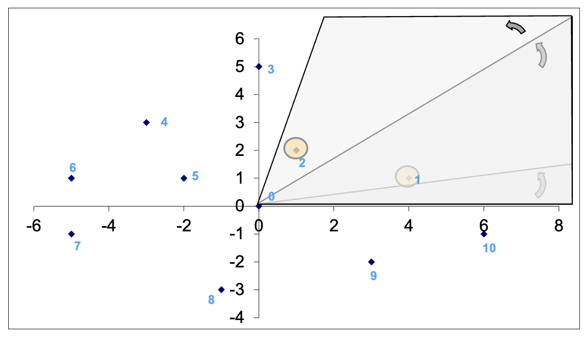
See slide 36 and 38 for an example solution.

Savings Method

The savings method is a heuristic for solving the VRP by iteratively merging routes based on the savings in distance achieved by combining them.

1. Start with each customer being served by a separate vehicle route.
2. Calculate the savings for each pair of customers $i$ and $j$ as (Clarke-Wright savings formula): $S_{ij}=d_{0i}+d_{0j}-d_{ij}$
   where $d_{0i}$ and $d_{0j}$ are the distances from the depot to customers $i$ and $j$, and $d_{ij}$ is the distance between customers $i$ and $j$.
3. Create a savings matrix that lists the savings for each pair of customers.
4. For each entry in the matrix, sorted by descending savings, check if they can be merged into a single route without violating vehicle capacity or other constraints. If they can be merged, combine their routes.
   • If a point is in the middle of a route, it cannot be merged with another route; only the first and last points are checked for possible merging.
5. Repeat step 4 until no more merges can be made.

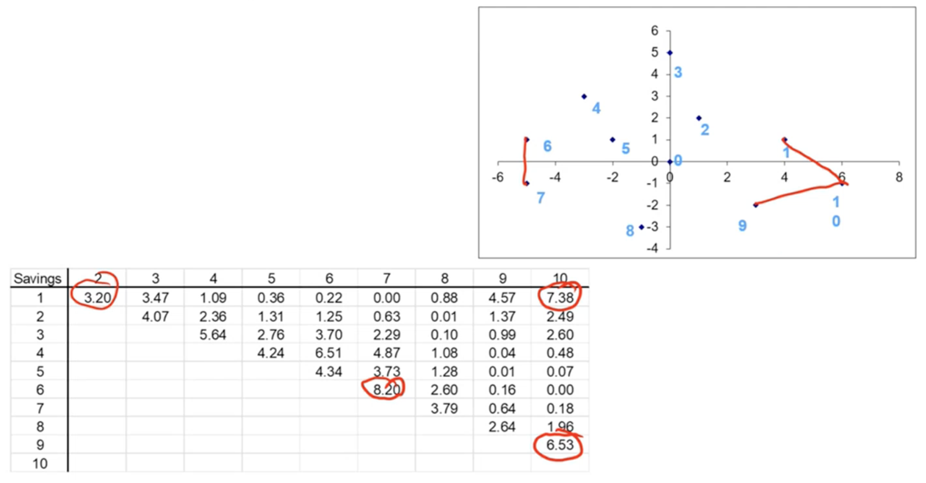
See slide 44 for an example solution.

Outlook: Complex Variants

Real-world, complex routing problems often include additional factors and constraints, such as road gradient, velocity (including traffic lights), acceleration, electric power and charging demand. They might also include additional objectives like minimizing emissions in addition to cost.