Resources

• Slides

Options

Options may be call or put and based on various underlying assets (financial instruments, commodities, indices, etc). Like Futures, they may be settled physically or in cash. Options are commonly used for hedging risk or for speculative purposes in financial markets.

• Call: The right to buy an asset at a predetermined price (strike price) within a specified time frame. When investors expect the underlying asset’s price to rise.
• Put: The right to sell an asset at a predetermined price (strike price) within a specified time frame. When investors expect the underlying asset’s price to fall.

Both calls and puts can be long (buying the option) or short (selling the option).

European options (commonly cash-settled) can only be exercised at expiration, while American options (commonly physical single-stock) can be exercised at any time before expiration.

Moneyness Levels

Different moneyness levels describe the relationship between the underlying asset’s price and the option’s strike price:

• At-the-Money (ATM): The underlying asset’s price is equal (or close) to the strike price.
• In-the-Money (ITM): For a call, the underlying asset’s price is above the strike price; for a put, the underlying asset’s price is below the strike price.
• Out-of-the-Money (OTM): For a call, the underlying asset’s price is below the strike price; for a put, the underlying asset’s price is above the strike price.

Option Value

The Option Value is the price of the option, which consists of two components (Option Value = Intrinsic Value + Time Value):

• Intrinsic Value: The difference between the underlying asset’s price and the strike price, representing the immediate exercise value of the option.
• Time Value: The additional value of the option due to the time remaining until expiration.

For call options, the value is:

$$C_0=S_0+P_0-K{q}^{-T}=\underset{\text{Intrinsic Value}}{\underbrace{S_0-K}}+\underset{\text{Time Value}}{\underbrace{P_0+K(1-q^{-T})}}$$

And for put options, the value is:

$$P_0=K{q}^{-T}-S_0+C_0=\underset{\text{Intrinsic Value}}{\underbrace{K-S_0}}+\underset{\text{Time Value}}{\underbrace{C_0-K(1-q^{-T})}}$$

See Pricing for factors that affect option value.

Payoffs

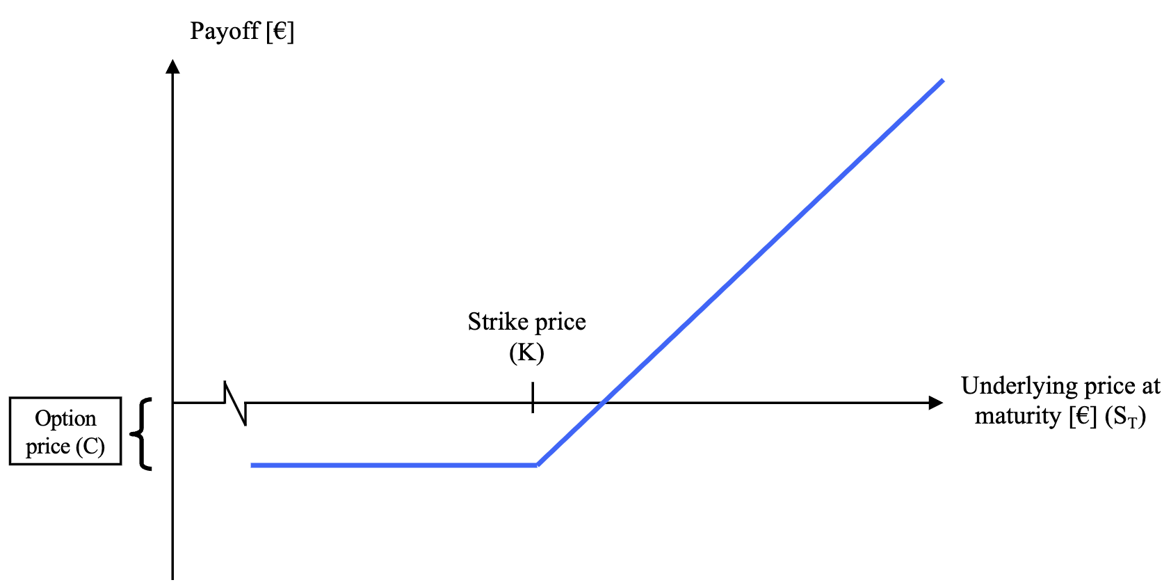
Long Call Payoffs

With a long call, the profit is theoretically unlimited, while the loss is limited to the purchase price (premium).

$$C_T=\max (S_T-K,0)$$

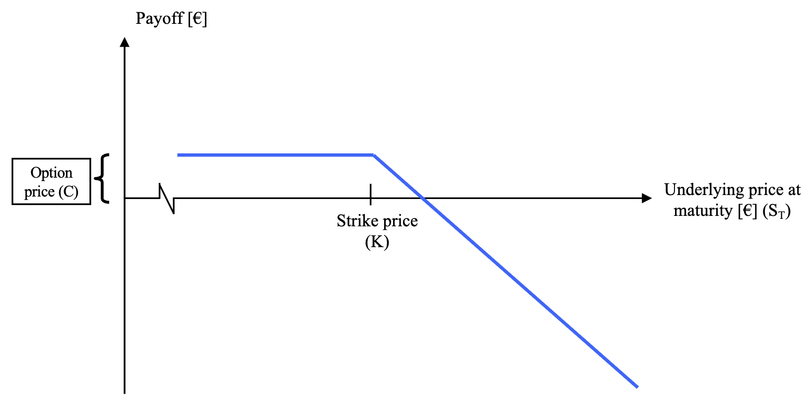
Short Call Payoffs

With a short call, the profit is limited to the premium received, while the loss is theoretically unlimited.

$$-C_T=\min (S_T-K,0)$$

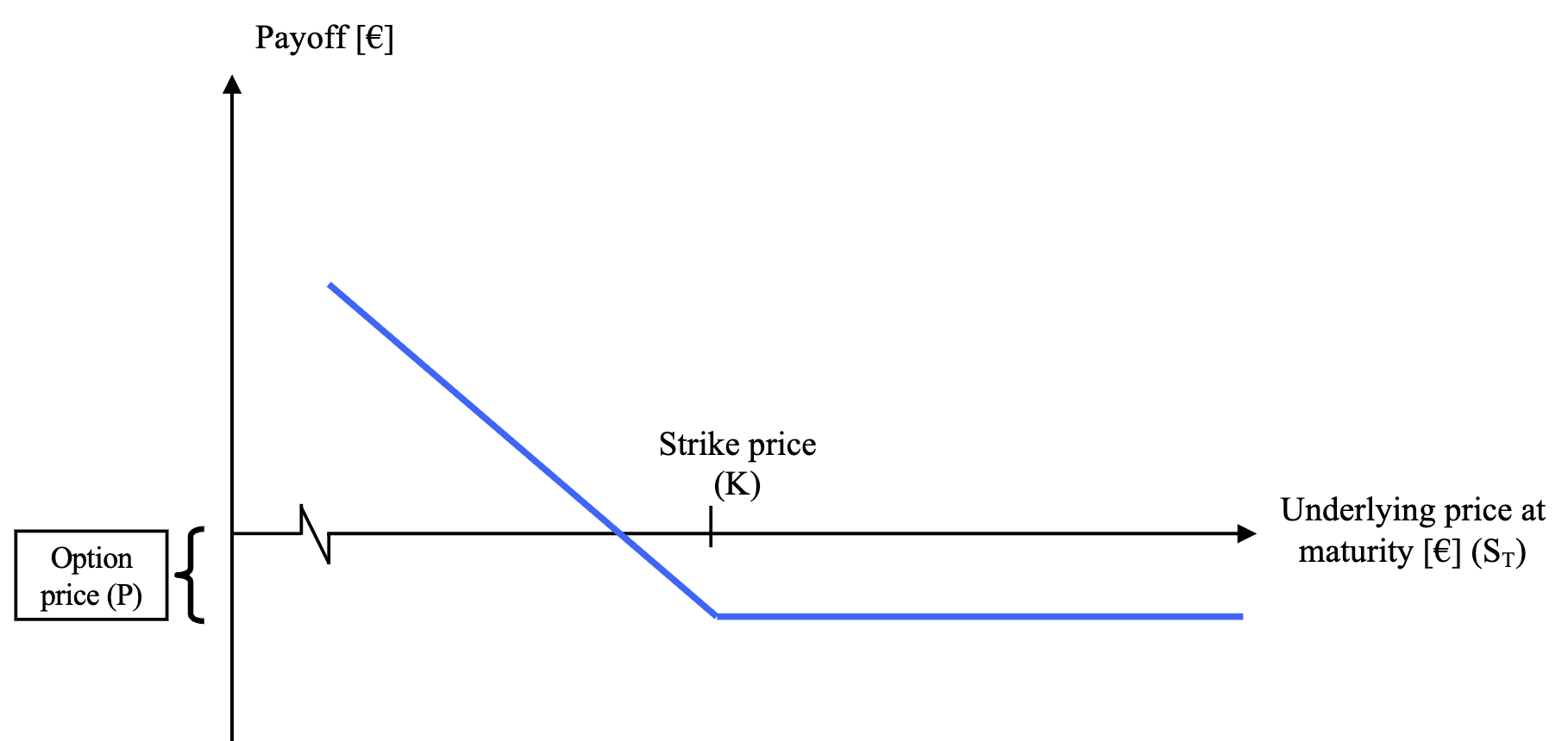
Long Put Payoffs

With a long put, the profit is limited to the exercise price minus the premium paid, while the loss is limited to the premium paid.

$$P_T=\max (K-S_T,0)$$

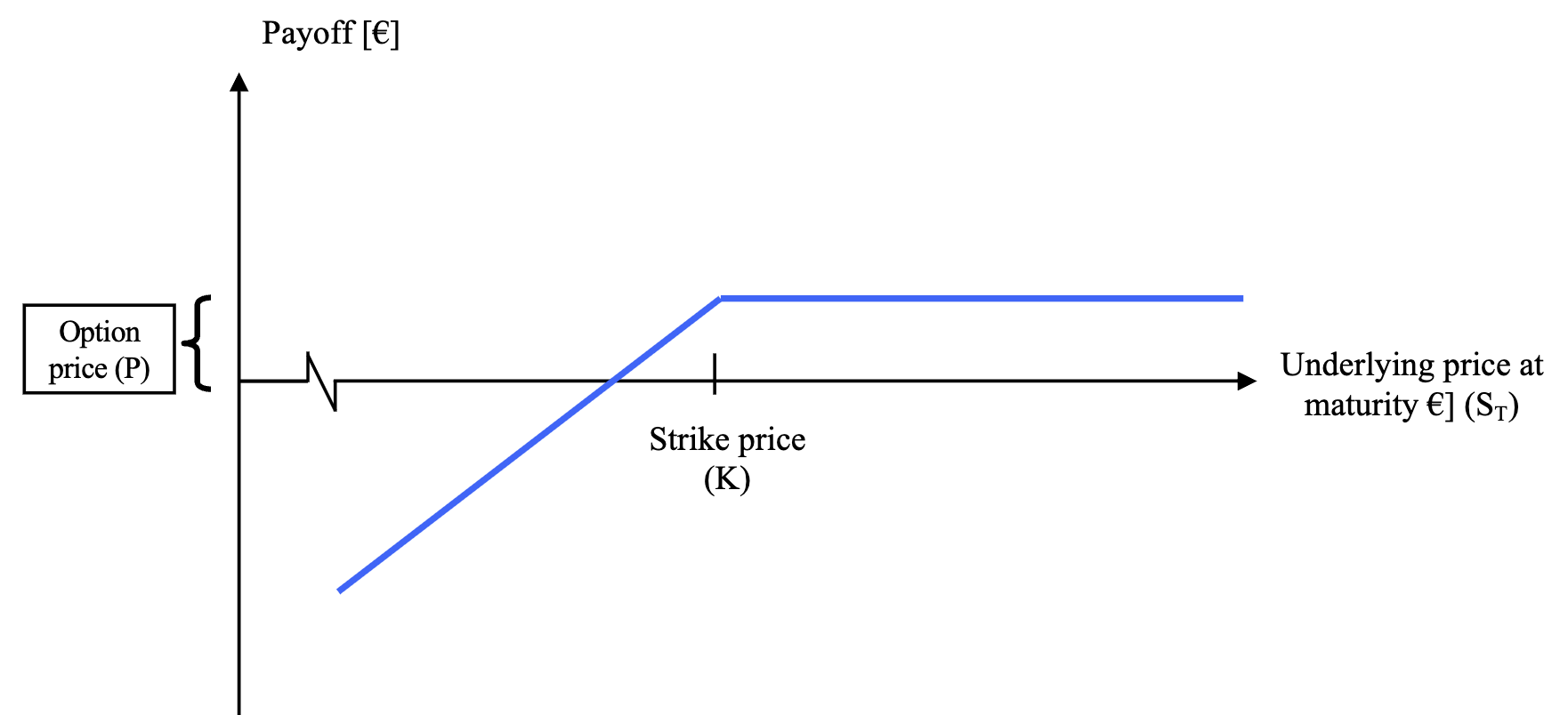
Short Put Payoffs

With a short put, the profit is limited to the premium received, while the loss is limited to the exercise price minus the premium received.

$$-P_T=\min (K-S_T,0)$$

Pricing

• Call options can never be worth more than the share itself: $C_t\le S_t$
• Put options can never be worth more than the strike price: $P_t\le K$
• An American option is always worth as least as much as a European option (same cash flows but additional flexibility). However, for call options on non-dividend paying stocks, early exercise is never optimal, so the American and European call option prices are equal.

The price is determined by several factors (see Option Value for the decomposition into intrinsic and time value):

Factor (Increases)	Call	Put
Underlying price S	+	-
Strike price K	-	+
Maturity T (European)	?	?
Maturity T (American)	+	+
Volatility	+	+
Risk-free interest rate	+	-
Expected future dividends	-	+

Put-Call Parity

When combining put and call options in a way that creates a risk-free portfolio, the riskless payout dictates what the portfolio must cost today to prevent arbitrage.

$S_0+P_0-C_0=K{q}^{-T}$

• Replication: A long stock combined with a long put and a short call perfectly replicates a risk-free zero-coupon bond with a face value of $K$.
• Arbitrage-Free: If the equation does not hold, traders can lock in riskless profits by buying the underpriced side and shorting the overpriced side.
• Directional Neutrality: The final payoff is always exactly $K$, completely independent of whether the stock price goes up, down, or stays flat.

Binomial Model

While the Block-Scholes model is widely used for pricing options, the binomial model is a simpler approach to option pricing by assuming the underlying asset price follows a binary path over a discrete period. It can also be used to represent dividends or other rights of the underlying asset by adjusting the stock price at each node.

Hedge Ratio

To value an option without needing to know the physical probability of an upward movement ($q$) or investors’ risk preferences, we construct a risk-free hedge portfolio. This portfolio consists of:

• Long: One share of the underlying asset ($S$).
• Short: $m$ call options on that asset ($C$).

For the portfolio to be completely risk-free, its payoff must be identical whether the stock moves up ($u$) or down ($d$):
$uS-m{C}_u=dS-m{C}_d$

Solving for $m$ gives the hedge ratio:
$m=\frac{uS-dS}{C_u-C_d}$

Risk-Neutral Valuation

Because this hedge portfolio is entirely risk-free, it must earn the risk-free interest rate ($r_f$), behaving exactly like a zero-coupon bond:
$(1+r_f)(S-mC)=uS-m{C}_u$

By substituting the hedge ratio into this equilibrium condition, we can isolate the current value of the option ($C$). This yields the fundamental pricing formula:

$C=\frac{p{C}_u+(1-p)C_d}{1+r_f}$

Where $p$ represents the risk-neutral probability of an upward movement:
$p=\frac{(1+r_f)-d}{u-d}$

Concept

The option value is simply the present value of its expected future payoffs. We calculate this expected value using the risk-neutral probability $p$, which mathematically embeds the market’s true risk aversion by underestimating the physical probability $q$ (effectively overestimating the “bad state”).

The expanded form explicitly shows how the valuation bypasses subjective expectations and relies solely on directly observable market variables ($u,d,r_f$):

$C=\frac{1}{1+r_f}\left[C_u\left(\frac{(1+r_f)-d}{u-d}\right)+C_d\left(\frac{u-(1+r_f)}{u-d}\right)\right]$

Multiple Periods

When extending the binomial model to multiple stages (e.g., a two-period model), the underlying asset price splits multiplicatively over successive intervals, creating an expanding tree of potential future states. To determine the current option price, backward induction is used.

1. Calculate Terminal Payoffs: First, determine the option’s value at the final expiration date ($t=2$) for every final stock price node ($C_{uu}$, $C_{ud}$, $C_{dd}$) using the standard intrinsic value formula $\max (S_T-K,0)$.
2. Step Backward to Intermediate Nodes: Use these terminal payoffs to calculate the expected option values at the intermediate stage ($t=1$) for both the up-state ($C_u$) and down-state ($C_d$): $$\begin{array}{rl}{C}_u& =\frac{p{C}_{uu}+(1-p)C_{ud}}{1+r_f}\\ C_d& =\frac{p{C}_{du}+(1-p)C_{dd}}{1+r_f}\end{array}$$
3. Discount to Present Value: Finally, treat those intermediate values ($C_u,C_d$) as the next period’s payoffs to discount back one last step to find the current option value ($C_0$) at $t=0$.

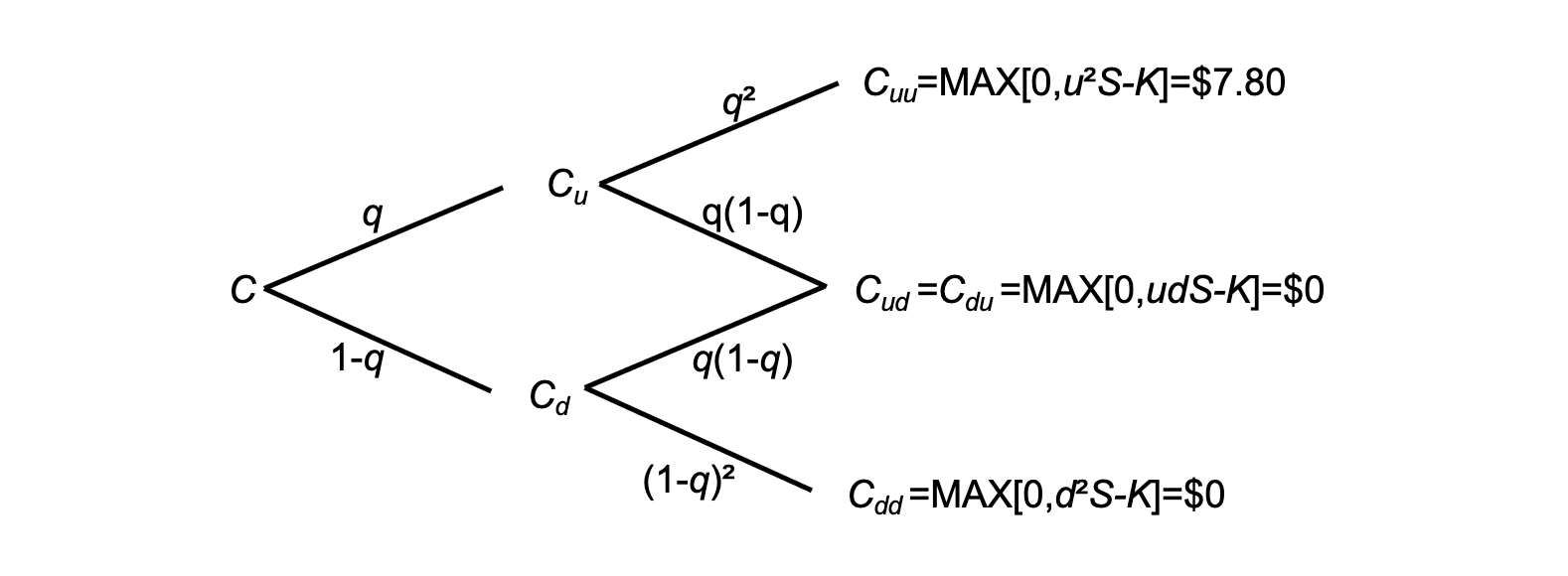
Models with a very large number of steps can be used to approximate the actual distribution of share prices, which is why the binomial model is often used in practice.

American Options & Early Exercise Boundary

To value an American option, the backward induction process requires an extra check at every node in the binomial tree:

• At each node, calculate the continuation value (the value of holding onto the option, derived via the standard risk-neutral discounted expected value).
• Compare this continuation value against the immediate intrinsic value if the investor were to exercise ($S_t-K$ for a call, or $K-S_t$ for a put).
• The true value assigned to that node is always the maximum of the two:
  $P_{\text{node}}=\max \left(\frac{p{P}_u+(1-p)P_d}{1+r_f},K-S_{\text{node}}\right)$

As mentioned above, American calls on non-dividend paying stocks are never exercised early, so their value is always equal to the European call value. For puts, however, early exercise can be optimal, especially when the option is deep in the money and interest rates are non-negative.