Resources

• Slides
• Exercise Questions (Solution)

If and how much of a product a company should order, to provide the required quantities of intermediate products, assemblies, and purchased parts on time for the production of end-products.

Inventory Management

Inventory is the stock of goods and materials held by a company to meet future demand.

• $\text{Net Inventory}=\text{Physical Inventory}-\text{Backlog}$
• $\text{Inventory Position (IP)}=\text{Net Inventory}+\text{Outstanding Orders}$

A positive inventory position indicates that the company has more stock than needed, while a negative inventory position indicates a shortage.

Key Costs

• Ordering Costs $A$: Costs incurred every time an order is placed, regardless of the order size (admin, shipping, setup).
• Holding Costs $h$: Costs associated with storing inventory over time (warehousing, insurance, depreciation, obsolescence).
• Shortage/Stockout Costs $p$: Costs incurred when demand cannot be met from inventory (lost sales, backorder costs, customer dissatisfaction).

Service Level Metrics

• Non-stockout probability $\alpha$: Share of periods without shortages
• Fill-Rate $\beta$: Share of demand fulfilled from stock immediately

Demand and Inventory Classification

• ABC Analysis: Categorization by consumption value (Pareto distribution; high, middle, low).
• XYZ Analysis: Categorization by demand regularity (steady, fluctuating, erratic/intermittent).
• ABC/XYZ Matrix: Combines both to identify core focus items (e.g., AX items).

ABC	XYZ
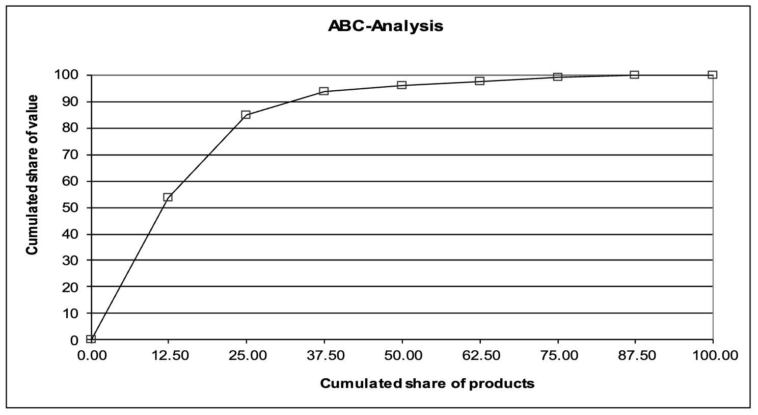Here, the first two products already account got 85% of value → A category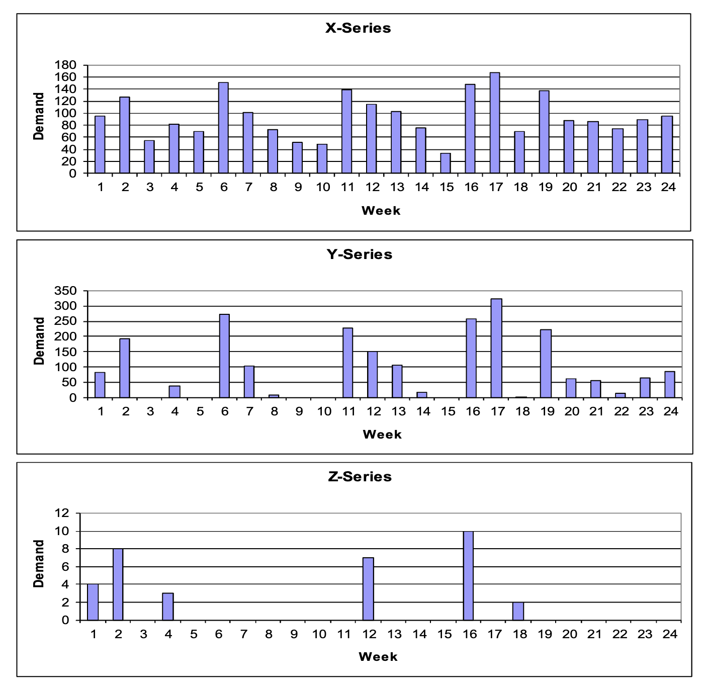

Continuous Inventory

In continuous inventory systems, inventory levels are continuously monitored, and orders are placed as soon as the inventory position reaches a predetermined reorder point. This approach allows for more responsive inventory management and can help prevent shortages.

Deterministic Lot-Sizing: The EOQ Model

The Economic Order Quantity model is used when demand is known and constant, and there are no lead times.

While not the most realistic decision tool, it’s a simple way to determine the optimal lot size to balance fixed ordering costs $A$ (low quantity → frequent orders) against holding costs $h$ (high quantity → high inventory).

Lot Size

Lot size is the quantity of a product that is either

• produced together, without interruption, in one production order
• procured in one common replenishment
• transported together

Inventory Development	Cost Function
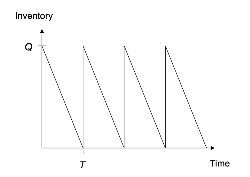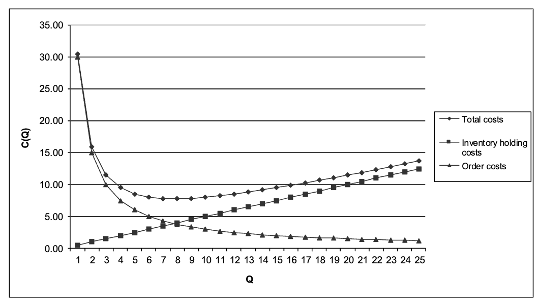	EOQ is at the minimum of total costs.

Assumptions

To stay simple, the EOQ model assumes:

• Continuous time and an infinite planning horizon
• Constant and known demand rate $d$ (units per time period)
• Procurement of materials in lots of size $Q$ at a fixed cost $A$ per order and at constant procurement costs $c$ per unit (e.g. purchase price)
• No lead time (instantaneous replenishment)
• Unlimited storage capacity with constant holding costs $h$ per unit and time period

Determining

The total cost per time unit is $C(Q)=\frac{d}{Q}\cdot A+\frac{h}{2}\cdot Q+c\cdot d$.
The optimality condition is therefore (first-order condition) $\frac{dC}{dQ}=-\frac{d}{Q^2}\cdot A+\frac{h}{2}=0$, which yields the solutions:

• Optimal Lot Size: $Q^{\ast }=\sqrt{\frac{2dA}{h}}$
• Optimal Order Interval: $T^{\ast }=\frac{Q^{\ast }}{d}=\sqrt{\frac{2A}{dh}}$
• Minimal Costs per Time Unit: $C^{\ast }=\sqrt{2dhA}+cd$

Economic Intuition at Q^*

Setting the derivative to zero proves that Total Fixed Ordering Costs equal Total Holding Costs at the optimum. This holds across three perspectives:

1. Per time unit: $\frac{d}{Q}\cdot A=\frac{h}{2}\cdot Q$ (ordering cost per time = avg holding cost per time)
2. Per unit: $\frac{A}{Q}=\frac{h}{2}\cdot \frac{Q}{d}$ (ordering cost per unit = avg holding cost per unit)
3. Per cycle: $A=\frac{h}{2}Q\cdot \frac{Q}{d}$ (fixed ordering cost = avg holding cost per cycle)

Stochastic Inventory Control Policies

Stochastic policies are used when demand is uncertain and lead times exist.

For each policy, the planning problem is setting the inventory control parameters to minimize costs under service level constraints.

Approximately, the parameters are set as follows:

• Period $R$ will be either fixed (e.g. at 1), or represent the classic economic order interval (EOI).
• Reorder point $s$ at the level of demand during the replenishment lead time, plus a safety stock: $s=d\cdot L+z\cdot {\sigma }_L$ (lead time times average demand, plus safety stock for the desired service level).
• Base stock level $S$ at the level of demand during the replenishment lead time (including review period), plus a safety stock.
• Quantity $Q$ at the economic order quantity (EOQ) level, which balances ordering and holding costs ($S-s=Q$).

$(R,S)$: Base-Stock Policy

In all $R$ periods (daily, monthly), the $(R,S)$ policy orders enough to bring the inventory position up to $S$ (by ordering $S-\text{IP}$). This policy is often used in continuous review systems.

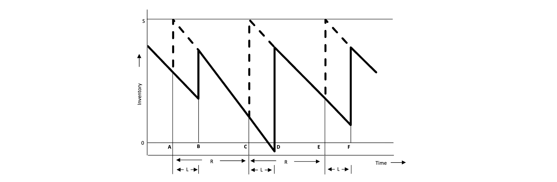
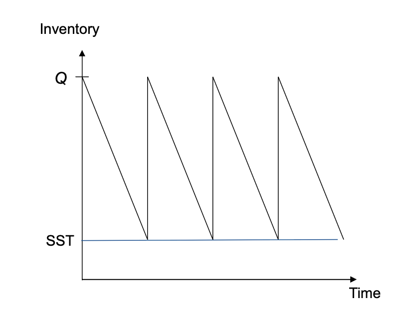
$(s,Q)$: Reorder Point: Order Quantity Policy

The $(s,Q)$ policy places an order of size $Q$ whenever the inventory position falls to/below a reorder point $s$. This helps maintain inventory levels within desired limits while accounting for demand variability.

$(s,S)$: Reorder Point: Order-Up-To Policy

The $(s,S)$ policy places an order to bring the inventory position up to $S$ whenever it falls to/below a reorder point $s$. This policy is often used in systems where order quantities can vary.

Single-Period Inventory

In single-period inventory problems, decisions are made for a single time period, and the goal is to balance the costs of ordering too much or too little inventory.

Applies to perishable, highly seasonal, or short-lifecycle goods (e.g., fashion, newspapers) where unsold inventory cannot be stored for long.

Newsvendor Model

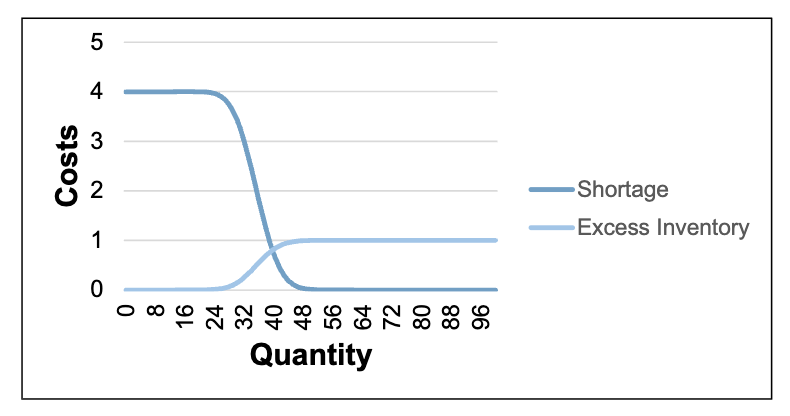
In this model, newsvendors need to order the right number of newspapers before knowing the actual demand. Ordering too many results in excess inventory, while ordering too few leads to missed sales. The optimal order quantity balances the expected costs of overstocking and understocking.

Both over- and understocking incur costs, so the optimal order quantity must balance these risks. However, the risk is asymmetric: the cost of understocking is usually higher than overstocking.

• Underage Cost $c_u$: Profit lost per unit missed ($p-c$).
• Overage Cost $c_o$: Loss incurred per unsold unit ($c-s$).

The ==optimal order quantity $y^{\ast }$== depends on the ratio of underage to overage costs and the cumulative distribution function $F(y)$ of demand:
$y^{\ast }=F^{-1}\left(\frac{c_u}{c_u+c_o}\right)$
$\frac{c_u}{c_u+c_o}$ is the cumulated probability of the demand distribution, or newsvendor fractile.

Critical Ratio

The critical ratio is the ratio of underage cost to the total cost of underage and overage:
$\text{Critical Ratio}=\frac{c_u}{c_u+c_o}$

• Ratio > 0.5: Penalty for missing sales is higher than for excess inventory → order more than the mean demand.
• Ratio < 0.5: Penalty for excess inventory is higher than for missing sales → order less than the mean demand.
• Ratio = 0.5: Equal penalty → order at the mean demand.

Normal Distribution

Under a normal distribution of demand, the optimal order quantity can be expressed in terms of the mean $\mu$ and standard deviation $\sigma$ of demand:
$y^{\ast }=\mu +z^{\ast }\cdot \sigma$
Here, $z^{\ast }$ is the safety factor determining how many standard deviations above the mean the order quantity should be set to achieve the desired service level. It’s the normal inverse cumulative distribution function at the critical ratio:
$z^{\ast }={\Phi }^{-1}\left(\frac{c_u}{c_u+c_o}\right)$
$\mu$ and $\sigma$ are simply the mean and standard deviation of the demand distribution, which can be estimated from historical data.

Simulation

In uncertain, dynamic, complex context, simulations are often used to evaluate inventory policies and their performance under different scenarios. This might be Monte-Carlo or event based simulations.

Inputs are stochastic variables like arriving customers, processing times, empirical and theoretical distributions, or random numbers.

Outputs are inventory levels/queues/services/costs, number of replications.

See slide152 onwards.

Kanban

Kanban is a visual scheduling system popular in lean manufacturing and just-in-time (JIT) production. It represents a pull approach, uses cards to indicate when new inventory should be produced or ordered.

When a full container is removed from storage, its Kanban card is put into a box (representing a production order). This card is then attached to the container with the next batch of parts.

The number of cards is therefore defined by average demand per unit $D$, replenishment time $RT$, safety factor $SF$, and container/lot size $Q$:
$M=\frac{D\cdot RT\cdot (1+SF)}{Q}$