Resources

• Slides
• Exercise Questions 1 (Solution), Exercise Questions 2 (Solution)

Where to place facilities and how to structure the movement of goods to customers to balance transportation, facility, and time costs.

Distribution Logistics

Structural Design

A distribution system’s structure is defined by its vertical and horizontal size:

• Vertical: Number of stages (plant warehouse → central warehouse → regional → fulfillment)
• Horizontal: Number of facilities at each stage

When evaluating a location, decisions balance:

• quantitative drivers: transportation, capacity costs, taxes
• qualitative drivers: infrastructure, stability

For innovation strategies, companies will expand existing and create new locations (geographic concentration vs. diversification). A variation/elimination strategy aims a partial closure (contraction) and aggregation (concentration). Rationalization means improving existing locations or relocating.

When selecting possible locations, a feasible solution is found using a scoring model on macro (country/region) or micro level. Promising locations are then evaluated using profitability and risk analysis.

Distance Measurement

Aside

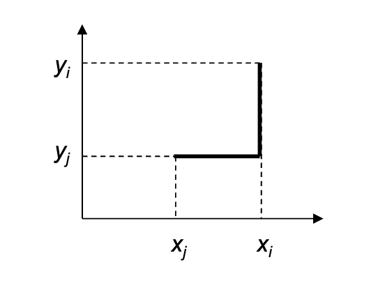
Rectangular Distance: Manhattan Metric

Distance is measured as the sum of the absolute differences in the horizontal and vertical coordinates, like in a grid street layout:

$d_{ij}=|x_i-x_j|+|y_i-y_j|$

Aside

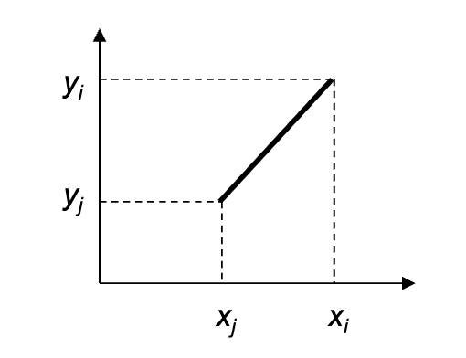
Euclidean Distance: Beeline

Distance is simply measured as the straight line between two points:
$d_{ij}=\sqrt{(x_i-x_j{)}^2+(y_i-y_j{)}^2}$

Real Distance: Road Network

Well, it’s the actual distance.

Continuous Location Planning: Steiner-Weber

Used to find the optimal $(u,v)$ coordinates on a map for a single facility without pre-defined candidate sites.

Each customer $j$ has a specific location $(x_j,y_j)$ and a demand quantity $b_j$ per time unit, with transport costs defined as $c$ per quantity and distance unit.

Weber's Location Theory

Weber theorized the optimal production location for a product with two sourcing location and one sales market:

• Both materials are ubiquitous → production near the market
• Two net weight materials → production near the market
• Two weight loss materials → tendency to the sourcing locations
• One ubiquitous, one weight loss → somewhere between weight loss and market

A net weight material is one that has negligent weight loss during production (fully used cotton), while a weight loss material loses weight (e.g., water or gases) during production due to waste, burning, or removing impurities.

The Steiner-Weber approach makes some important assumptions that limit its applicability:

• It exclusively considers linear transport costs while ignoring facility investment costs.
• It assumes all spatial coordinates are feasible without geographic constraints.
• It treats customer locations as static point demands rather than dynamic zones

$L_1$ Metric: Manhattan Distances

The goal is to minimize the weighted sum of Manhattan distances to all customers:
$\min F(u,v)=c\cdot {\sum }_{j=1}^n{b}_j\cdot \left(|u-x_j|+|v-y_j|\right)$

Because $u$ and $v$ coordinates are completed uncoupled in the Manhattan metric, the optimal location can be found by minimizing the weighted sum of distances in each dimension separately. This is done by sorting the customers by their $x$ and $y$ coordinates and finding the weighted median for each dimension, and the optimal location will always land on existing customer coordinates (customer $h$ for $u$ and $v$ each).

1. Calculate total demand $B={\sum }_j^n{b}_j$
2. Sort customers by $x$ coordinates ascending (such that $x_1\le x_2\le ...\le x_n$)
3. Find the coordinate $u^{\ast }=x_h$ where cumulative demand reaches/exceeds half of total demand for the first time (the weighted median): ${\sum }_{j=1}^{h-1}{b}_j<0.5\cdot B\text{and}{\sum }_{j=1}^h{b}_j\ge 0.5\cdot B$
4. Repeat the identical sorting and cumulative threshold procedure for y-coordinates to determine $v^{\ast }$.

$L_2$ Metric: Euclidean Distances

The goal is to minimize the weighted sum of Euclidean distances to all customers, which is a convex optimization problem:
$\min F(u,v)=c\cdot {\sum }_{j=1}^n{b}_j\cdot \sqrt{(u-x_j{)}^2+(v-y_j{)}^2}$

The optimal coordinates are coupled inside the root of the Euclidean distance function, so the optimal location has to be found iteratively using Weiszfeld’s iterative approximation:

1. Determine the initial center of gravity ($k=0$): $u^0=\frac{{\sum }_{j=1}^n{b}_j\cdot x_j}{{\sum }_{j=1}^n{b}_j},v^0=\frac{{\sum }_{j=1}^n{b}_j\cdot y_j}{{\sum }_{j=1}^n{b}_j}$
2. Iteratively update the coordinates until convergence ($k\to k+1$): $u^{k+1}=\frac{{\sum }_{j=1}^n\frac{b_j\cdot x_j}{\sqrt{(u^k-x_j{)}^2+(v^k-y_j{)}^2}}}{{\sum }_{j=1}^n\frac{b_j}{\sqrt{(u^k-x_j{)}^2+(v^k-y_j{)}^2}}},v^{k+1}=\frac{{\sum }_{j=1}^n\frac{b_j\cdot y_j}{\sqrt{(u^k-x_j{)}^2+(v^k-y_j{)}^2}}}{{\sum }_{j=1}^n\frac{b_j}{\sqrt{(u^k-x_j{)}^2+(v^k-y_j{)}^2}}}$
3. Repeat until the change in coordinates is below a small threshold $ϵ$.

Strategy: 5-Row Table Formula

For each customer $j\in \{A,B,C,D,E\}$, you just fill across the columns:

• $\Delta x$ & $\Delta y$: Subtract current location from customer coords $(x_j-u,y_j-v)$.
• $d_j$: $\sqrt{(\Delta x{)}^2+(\Delta y{)}^2}$
• Weight: $W_j=\frac{b_j}{d_j}$
• Weighted $x$: $W_j\cdot x_j$
• Weighted $y$: $W_j\cdot y_j$

Then sum up the last three columns and divide:
$u^{(\text{next})}=\frac{\sum (W_j\cdot x_j)}{\sum W_j},v^{(\text{next})}=\frac{\sum (W_j\cdot y_j)}{\sum W_j}$

This was not part of the lecture.

Discrete Location Planning: Warehouse Location Problem

The Warehouse Location Problem (WLP) addresses discrete network optimization, selecting facility sites and customer allocations to minimize total fixed and variable costs. Decisions are made on two levels:

• Strategic Level: Decides warehouse open/close decisions and macro customer assignments.
• Operational Level: Determines daily vehicle routing and multi-stop delivery tours.

To solve this problem, sequential planning (location→tours) is common, but it can lead to suboptimal solutions. Simultaneous planning (location+tours) is more complex but yields better results. Hierarchical planning (strategic location→tactical routing→operational delivery) balances complexity and solution quality by anticipating tour-dependent transportation costs.

The mixed-integer linear programming formulation of the WLP is as follows:

• $j\in \{1,\dots ,m\}$ customers with periodic demand $b_j$.
• $i\in \{1,\dots ,n\}$ candidate facility sites with fixed costs $f_i$ and capacity $a_i$.
• $c_{ij}$: Unit transport and production cost from facility $i$ to customer $j$
• $y_i\in \{0,1\}$: Binary decision variable indicating if facility $i$ is opened.
• $x_{ij}\ge 0$: Decision on quantity shipped from facility $i$ to customer $j$.

$$\begin{array}{rlr}\min Z& =\sum _{i=1}^n{f}_i\cdot y_i+\sum _{i=1}^n\sum _{j=1}^m{c}_{ij}\cdot x_{ij}& \\ \text{s.t.}\sum _{i=1}^n{x}_{ij}& =b_j\forall j\in \{1,\dots ,m\}& \text{(Demand)}\\ \sum _{j=1}^m{x}_{ij}& \le a_i\cdot y_i\forall i\in \{1,\dots ,n\}& \text{(Capacity)}\\ x_{ij}& \ge 0,y_i\in \{0,1\}\forall i,j& \end{array}$$

This might be solved using the branch and bound method or heuristics.

Add Heuristic Solution Method

When exact methods (Branch and Bound) are too slow, the Add Heuristic builds a solution construct:

1. Initial Step: Find and open the single candidate location $i$ that minimizes total costs (fixed costs plus transport costs to serve all customers).
2. Iterative Step: For each remaining closed site, calculate potential savings in transportation costs if that site were opened. This is the sum of savings for all customers where shipping from the new candidate site is cheaper. Subtract the site’s fixed cost $f_i$ from the gross transport savings.
   • Selection: Open the site yielding the highest net positive savings. Sites with a negative net savings are forbidden.
3. Termination: Repeat until no unopened candidate site yields a positive net cost reduction. All sites should be either opened or forbidden.

Discrete Location Planning: Set Covering Problem

The Set Covering Problem focusses on achieving complete coverage of a target population or area using the minimum number of resources. In contrast to the WLP, which balances fixed and variable costs, the Set Covering Problem emphasizes coverage efficiency (time or service).

An example are time-focussed models, where all customers need to be served within a certain time window, or emergency service, where a limited number of stations must be placed to ensure all locations are covered.

The SCP can be approached from two directions:

• Problem 1: Minimize the number of required locations, under the constraint that all customers must be served within a given time/distance.
• Problem 2: Maximize the number of customers that can be attracted with a given number of locations.

$N(i$) is the set of locations that fulfill customer $i$‘s service taget (out of $I$, the set of customers and $J$, the set of locations, given a maximum distance of $S$): $N(i)=\{j\in J\mid d_{ij}\le S\}$

The lecture does not cover any heuristics to solve these, instead the model formulations can simply be given to a solver:

Problem 1: Location Minimization

$\begin{array}{rlr}\min & \sum _{j\in J}{x}_j& \\ \text{s.t.}& \sum _{j\in N(i)}{x}_j\ge 1,& \forall i\in I\\ & x_j\in \{0,1\},& \forall j\in J\end{array}$

Problem 2: Customer Maximization

$\begin{array}{rlr}\max & \sum _{i\in I}{a}_i{y}_i& \\ \text{s.t.}& \sum _{j\in N(i)}{x}_j\ge y_i,& \forall i\in I\\ & \sum _{j\in J}{x}_j=p,& \\ & x_j\in \{0,1\},& \forall j\in J\\ & y_i\in \{0,1\},& \forall i\in I\end{array}$
Where $a_i$ is the weight of customer $i$ (e.g., population, demand, or priority) and $p$ is the maximum number of locations that can be opened.

Network Structures

Network design is a weighing of the number of nodes/links (minimizing the length of the network) against the number of transshipments (minimizing handling and lead time) and political discussions (advantages of, e.g., public infrastructure).

• Direct Transports: Point-to-point routes between origin $A$ and destination $Z$ without intermediate handling. This requires the most links.
• Relay Traffic: Drivers/vehicles start at opposing ends $A$ and $Z$, meet midway at $B$ to swap trailers, and return.
• Hub-and-Spoke: Centralizes collection, sorting, and distribution to aggregate flows across many origin-destination pairs.
• Cross-Docking: Incoming shipments are transferred directly to outbound transport with minimal or no interim storage. Objectives are transport consolidation and shorter lead times.

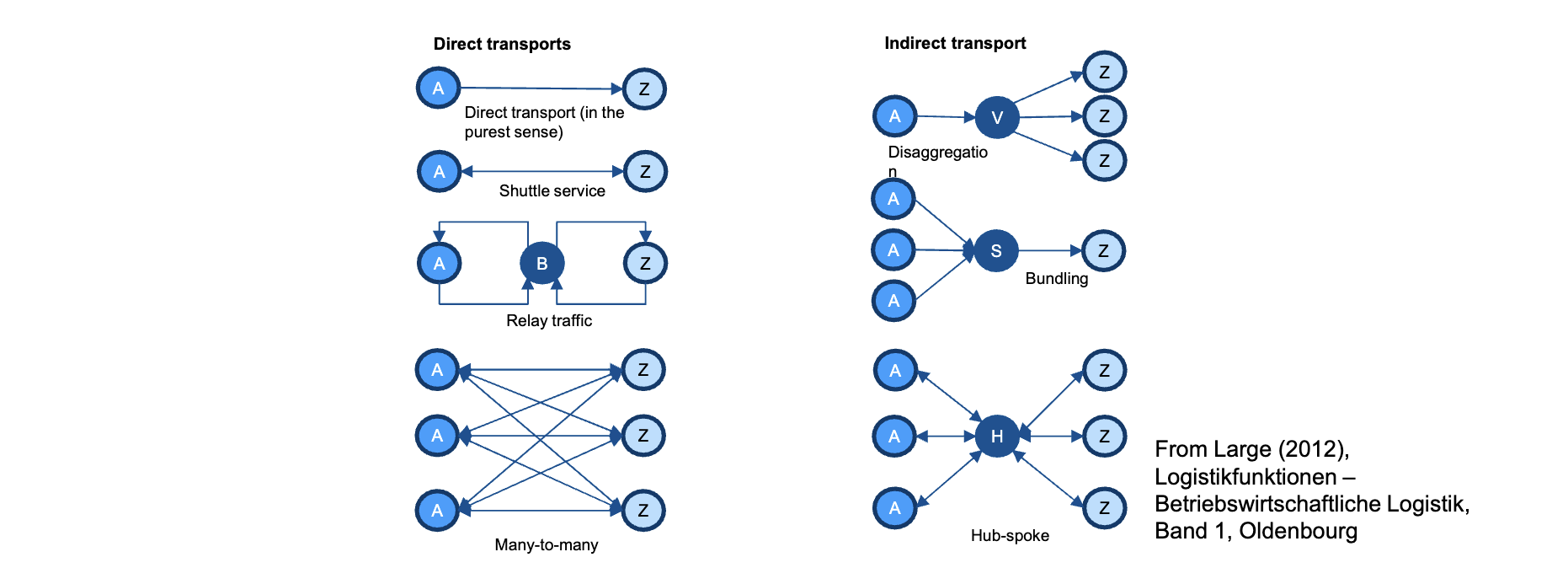
Disaggregation means breaking down large shipments into smaller ones for local delivery; Bundling consolidates freight to achieve economies of scale.

The Postponement Strategy delays final product differentiation until exact demand is known (e.g., Benetton knitting garments before dyeing them).

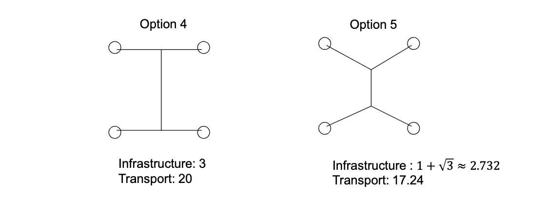
Example: infrastructure and transportation costs for connecting 4 points in a square with a side length of 1 and exchange quantities of 1:

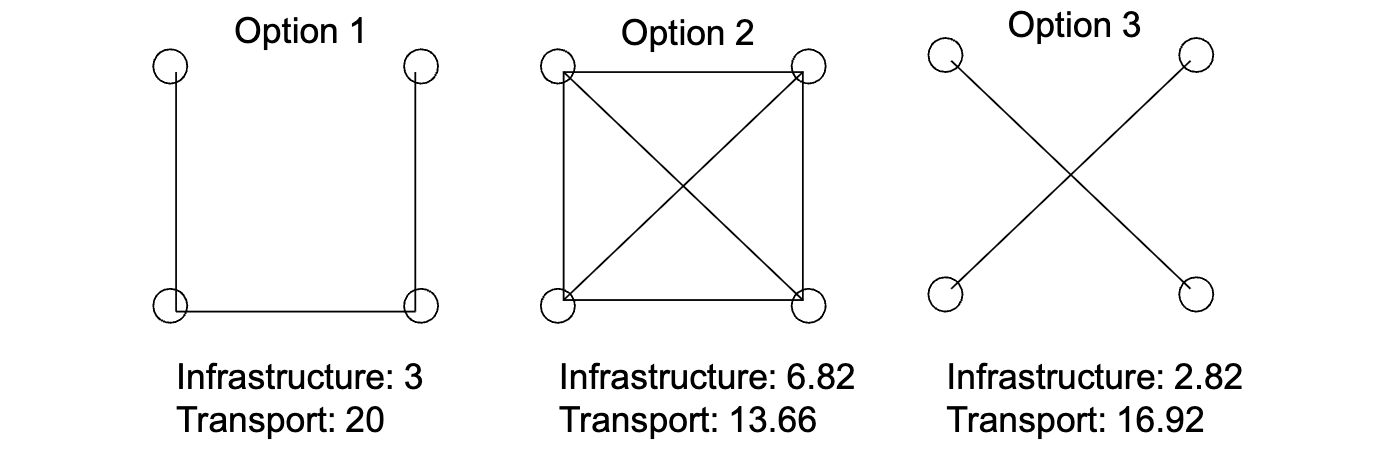
Network Distance Formulae

Not sure if this was just meant as an example or if there will be a question like this in the exam.

For $n$ nodes spaced uniformly around a circle of radius $r$, delivering 1 unit between every node pair:

Network Configuration	Distance Formula (n even)	Distance Formula (n odd)
Individual Transport	$Z=2r\pi \cdot n$	same
Central Hub	$Z=2r\cdot n$	same
Cross-Docking (Separated)	$Z=2r\cdot (n+1)+2r\pi \frac{n-1}{n}$	$Z=r\pi \cdot n$
Decentral Hub Cross-Dock	$Z=4\cdot \frac{2r\pi }{n}\left(1+2+\cdots +\frac{n-1}{2}\right)$	$Z=\frac{r\pi }{n}(n-1)(n+1)$